Big-O Notation - How Your Code Behaves at Scale

In 2012, a developer at a startup wrote a 50-line function to check for duplicate users during registration. It worked perfectly in testing with 500 users. Each check completed in milliseconds.

When they launched and hit 50,000 users, the registration endpoint started timing out occasionally. At 500,000 users, the entire system froze during peak registration hours. The backend team spent two weeks investigating. They blamed the database. They blamed the network. They added more servers.

The problem was a 50-line Python function. The function compared each new user against every existing user - an O(n²) algorithm. With 500 users: 250,000 comparisons per registration. With 500,000 users: 250,000,000,000 comparisons. The server was not slow. The algorithm was catastrophically wrong.

The fix: three lines using a set lookup. O(n) space, O(1) per lookup. Registration time: unchanged regardless of how many users existed.

The lesson: correct code that does not scale is not production-ready code. Big-O is the tool for knowing the difference before you ship.

What You Will Learn

• What Big-O measures and why it matters more than raw speed
• O(1) constant time: operations that stay fast regardless of data size
• O(n) linear time: operations that scale proportionally
• O(n²) quadratic time: the hidden danger in nested loops
• O(log n) logarithmic time: why binary search handles a million elements in 20 steps
• O(2^n) exponential time: why naive recursion explodes and how memoization saves it
• How to compare all complexity classes with a single visualization
• Best, worst, and average case analysis
• Space complexity and the time-space tradeoff
• Why testing with small inputs lies to you

Prerequisites

• You have written Python loops (for, while), conditionals, functions, and recursion
• You understand that dictionaries use hash tables (lookup is different from list search)
• You have encountered timeit or measured code performance at least once

Mental Model: The Growth Question

Big-O does not answer "how fast is this code?"

Big-O answers "if I double the input size, what happens to the runtime?"

Input size doubled:
                                    Runtime when n doubles:
O(1)     - stays the same          1ms → 1ms   (no change)
O(log n) - increases slightly      1ms → 1.something ms
O(n)     - doubles                 1ms → 2ms
O(n log n) - slightly more than double  1ms → ~2.1ms
O(n²)    - quadruples              1ms → 4ms
O(2^n)   - squares                 1ms → 1,000,000ms (explodes)

This is why O(n²) code passes all your unit tests but destroys production. At n=10, O(n²) feels instant. At n=10,000, it is 1 million times slower than O(n).

Part 1 - The Question Big-O Answers

Big-O is not about absolute speed. Absolute speed depends on hardware, OS, Python version, and a hundred other factors.

Big-O is about growth rate - how runtime grows as input grows.

Define n as the input size:

• Processing a list of 1,000 items: n = 1,000
• Searching a database of 10 million users: n = 10,000,000
• Training a model on 100 million examples: n = 100,000,000

The question is always: "As n grows, how does work grow?"

The mathematical notation O(f(n)) means "runtime grows proportionally to f(n)". Constants and lower-order terms are dropped:

• 3n + 7 → O(n) (the 3 and 7 don't matter at large n)
• n² + 100n → O(n²) (the 100n term is irrelevant compared to n²)
• 5 → O(1) (constant regardless of n)

tip

Big-O describes the dominant term as input grows to large values. A function that takes 100n + n² operations is O(n²) because at large n, the n² term overwhelms the 100n term. Drop constants, drop lower-order terms, keep the dominant growth.

Part 2 - O(1) - Constant Time

O(1) operations complete in the same amount of time regardless of input size. Accessing the millionth element of a list is as fast as accessing the first element. This is the property that makes certain data structures powerful.

O(1) operations in Python:

import timeit

# Dictionary lookup - O(1) regardless of dictionary size
my_dict = {str(i): i for i in range(1_000_000)}

time_small = timeit.timeit(lambda: my_dict["500"], number=100_000)
time_large = timeit.timeit(lambda: my_dict["999999"], number=100_000)
# Output: both times are nearly identical - O(1) confirmed

# List index access - O(1)
my_list = list(range(1_000_000))
print(my_list[0])          # First element - immediate
print(my_list[999_999])    # Last element - equally immediate
# Output: 0 and 999999 - same speed

# Set membership test - O(1) (amortized)
my_set = set(range(1_000_000))
print(999_999 in my_set)   # True - O(1), not O(n)
print(2_000_000 in my_set) # False - O(1), not O(n)

# List append (amortized O(1))
items = []
items.append("new_item")   # O(1) amortized - occasionally O(n) for resize
                           # but average over many appends is O(1)

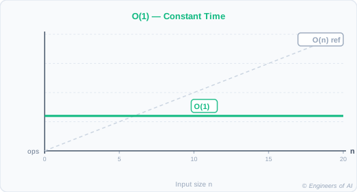
A flat line. Doubling n changes nothing.

Why this matters in production: A membership check called a million times per second must be O(1). Using a set instead of a list for membership checks is one of the highest-value, lowest-effort performance improvements in Python. The fix is often one character: [] → {} or set().

Part 3 - O(n) - Linear Time

O(n) operations grow proportionally with input. Double the input, double the time. This is predictable and manageable - for most data sizes, O(n) algorithms are perfectly acceptable.

O(n) operations in Python:

import time

def sum_list(numbers):
    """O(n) - must visit every element once"""
    total = 0
    for number in numbers:   # Executes n times
        total += number
    return total

def find_first_even(numbers):
    """O(n) worst case - might stop early, but worst case checks all n elements"""
    for number in numbers:
        if number % 2 == 0:
            return number
    return None

# Demonstrate linear growth
for n in [1_000, 10_000, 100_000, 1_000_000]:
    data = list(range(n))
    start = time.perf_counter()
    result = sum_list(data)
    elapsed = time.perf_counter() - start
    print(f"n={n:>10,}: {elapsed*1000:.4f}ms")

# Output (approximate - varies by machine):
# n=     1,000: 0.05ms
# n=    10,000: 0.50ms    ← ~10x more work, ~10x more time
# n=   100,000: 5.00ms    ← ~10x more work, ~10x more time
# n= 1,000,000: 50.00ms   ← ~10x more work, ~10x more time

O(n) built-in Python functions:

numbers = list(range(1_000_000))

max(numbers)       # O(n) - must check every element
min(numbers)       # O(n) - must check every element
sum(numbers)       # O(n) - must add every element
sorted(numbers)    # O(n log n) - NOT O(n), see Part 7

# List search is O(n) - this is why sets exist
target = 999_999
if target in numbers:  # O(n) - checks up to n elements
    print("found")

# Contrast: set search is O(1)
numbers_set = set(numbers)
if target in numbers_set:  # O(1)
    print("found")

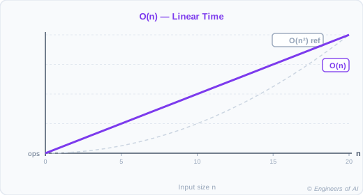
A straight diagonal line. Proportional growth.

Part 4 - O(n²) - Quadratic Time

O(n²) algorithms contain nested loops over the same data. When you double the input, the work quadruples. This is the class of algorithm that passes small-scale tests and destroys production systems.

The duplicate user bug from the hook:

import time

# O(n²) approach - the startup's original bug
def has_duplicates_slow(users):
    """Check if any two users share the same email.
    DANGER: O(n²) - compares every user to every other user"""
    for i in range(len(users)):
        for j in range(len(users)):   # Inner loop: runs n times for each outer iteration
            if i != j and users[i]["email"] == users[j]["email"]:
                return True
    return False

# O(n) approach - the 3-line fix
def has_duplicates_fast(users):
    """O(n) - each user visited once, set lookup is O(1)"""
    seen_emails = set()
    for user in users:
        if user["email"] in seen_emails:  # O(1) lookup
            return True
        seen_emails.add(user["email"])    # O(1) insert
    return False

# Demonstrate the catastrophic difference
for n in [100, 1_000, 5_000, 10_000]:
    users = [{"email": f"user{i}@example.com"} for i in range(n)]

    start = time.perf_counter()
    has_duplicates_slow(users)
    slow_time = time.perf_counter() - start

    start = time.perf_counter()
    has_duplicates_fast(users)
    fast_time = time.perf_counter() - start

    print(f"n={n:>6}: slow={slow_time*1000:.1f}ms, fast={fast_time*1000:.2f}ms, ratio={slow_time/fast_time:.0f}x")

# Output (approximate):
# n=   100: slow=0.5ms,    fast=0.01ms,  ratio=50x
# n= 1,000: slow=45ms,     fast=0.05ms,  ratio=900x
# n= 5,000: slow=1100ms,   fast=0.25ms,  ratio=4400x
# n=10,000: slow=4400ms,   fast=0.50ms,  ratio=8800x

Operations count comparison:

n	O(n) operations	O(n²) operations	Ratio
100	100	10,000	100x
1,000	1,000	1,000,000	1,000x
10,000	10,000	100,000,000	10,000x
1,000,000	1,000,000	1,000,000,000,000	1,000,000x

At 1 million items: O(n) takes seconds, O(n²) takes weeks.

The O(n²) pattern to recognize:

# PATTERN: nested loop where both iterate over the same n items
for i in range(n):        # n iterations
    for j in range(n):    # n iterations × n outer = n² total
        # work here

# COMMON MISTAKE: assuming this is O(n) because "it's just two loops"
for item in data:
    for other_item in data:     # n × n = n² - this is O(n²)
        if item != other_item:
            compare(item, other_item)

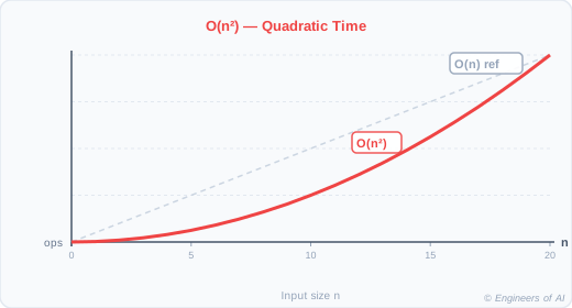
A steep curve that rises rapidly.

danger

An O(n²) algorithm that works fine at n=1,000 will be 10,000x slower at n=100,000. This is not a performance degradation - it is a system collapse. Always benchmark algorithms with the production data size, not the development data size.

Part 5 - O(log n) - Logarithmic Time

O(log n) algorithms halve the problem with each step. They are among the most powerful algorithms in engineering because they handle enormous inputs with surprisingly few operations.

The intuition: halving a million takes only 20 steps

log₂(1,000,000) = 19.9 ≈ 20

Starting from 1,000,000 items, halving 20 times reaches 1 item. That is why binary search on a sorted list of a million items takes at most 20 comparisons.

The "Guess My Number" analogy:

I am thinking of a number between 1 and 1,000.
You can ask YES/NO questions.

Naive strategy (O(n)): "Is it 1? Is it 2? Is it 3?..." - up to 1,000 questions
Binary strategy (O(log n)): "Is it > 500? Is it > 750? Is it > 875?..." - at most 10 questions

log₂(1,000) ≈ 10

Even with 1,000,000 numbers, binary search needs at most 20 questions.

Binary search implementation:

def binary_search(sorted_list, target):
    """O(log n) - halves the search space with each comparison"""
    low = 0
    high = len(sorted_list) - 1
    steps = 0

    while low <= high:
        steps += 1
        mid = (low + high) // 2

        if sorted_list[mid] == target:
            print(f"Found in {steps} steps")
            return mid
        elif sorted_list[mid] < target:
            low = mid + 1    # Discard left half
        else:
            high = mid - 1   # Discard right half

    print(f"Not found after {steps} steps")
    return -1

# Demonstrate O(log n) steps
import math

for n in [100, 1_000, 10_000, 1_000_000, 1_000_000_000]:
    sorted_data = list(range(n))
    target = n - 1  # Worst case: target at the end

    print(f"\nn={n:>12,}: theoretical max steps = {math.ceil(math.log2(n))}")
    binary_search(sorted_data, target)

# Output:
# n=         100: theoretical max steps = 7
# Found in 7 steps
#
# n=       1,000: theoretical max steps = 10
# Found in 10 steps
#
# n=      10,000: theoretical max steps = 14
# Found in 14 steps
#
# n=   1,000,000: theoretical max steps = 20
# Found in 20 steps
#
# n=1,000,000,000: theoretical max steps = 30
# Found in 30 steps

Comparison: linear search vs binary search at scale

import time
import bisect

# Linear search: O(n)
def linear_search(items, target):
    for i, item in enumerate(items):
        if item == target:
            return i
    return -1

# Binary search: O(log n)  - requires sorted input
def binary_search_fast(sorted_items, target):
    index = bisect.bisect_left(sorted_items, target)
    if index < len(sorted_items) and sorted_items[index] == target:
        return index
    return -1

n = 1_000_000
data = list(range(n))
target = n - 1  # Worst case for linear search

start = time.perf_counter()
linear_search(data, target)
linear_time = time.perf_counter() - start

start = time.perf_counter()
binary_search_fast(data, target)
binary_time = time.perf_counter() - start

print(f"Linear search (O(n)):    {linear_time*1000:.2f}ms")
print(f"Binary search (O(log n)): {binary_time*1000:.4f}ms")
print(f"Binary is {linear_time/binary_time:.0f}x faster")

# Output (approximate):
# Linear search (O(n)):     48.30ms
# Binary search (O(log n)):  0.002ms
# Binary is 24,000x faster

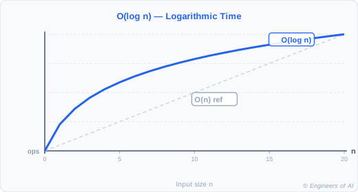
Fast rise then nearly flat - diminishing returns on additional input.

Part 6 - O(2^n) - Exponential Time

O(2^n) algorithms double the work with each additional input element. They are appropriate for problems where you must examine all possible combinations - but extremely dangerous when applied to the wrong problem.

The naive Fibonacci disaster:

import functools
import time

# NAIVE O(2^n) - exponential explosion
def fib_naive(n):
    """Each call spawns two more calls. The call tree doubles in size each step."""
    if n <= 1:
        return n
    return fib_naive(n - 1) + fib_naive(n - 2)  # Two recursive calls per invocation

# Count the actual number of function calls
call_count = [0]

def fib_counted(n):
    call_count[0] += 1
    if n <= 1:
        return n
    return fib_counted(n - 1) + fib_counted(n - 2)

for n in [5, 10, 20, 30]:
    call_count[0] = 0
    result = fib_counted(n)
    print(f"fib({n:>2}) = {result:>8,}  |  function calls: {call_count[0]:>10,}")

# Output:
# fib( 5) =        5  |  function calls:         15
# fib(10) =       55  |  function calls:        177
# fib(20) =    6,765  |  function calls:     21,891
# fib(30) =  832,040  |  function calls:  2,692,537

At fib(30): 2.7 million calls to compute one number. At fib(50): approximately 2.25 × 10¹⁰ calls - takes hours on modern hardware. At fib(100): essentially impossible.

Visualizing the call tree for fib(5):

                   fib(5)
                  /       \
           fib(4)           fib(3)
          /     \          /     \
       fib(3)  fib(2)   fib(2)  fib(1)
       /   \   /   \   /   \
    fib(2) fib(1) fib(1) fib(0) fib(1) fib(0)
    /   \
 fib(1) fib(0)

fib(3) is computed TWICE
fib(2) is computed THREE times
fib(1) is computed FIVE times

Every redundant computation is exponential waste. The fix: memoization.

O(n) fix with memoization (dynamic programming):

# MEMOIZED O(n) - each unique fib(k) computed exactly once
@functools.lru_cache(maxsize=None)
def fib_memo(n):
    """Each fib(k) computed once, stored in cache. n unique computations total."""
    if n <= 1:
        return n
    return fib_memo(n - 1) + fib_memo(n - 2)

# Comparison: naive vs memoized
for n in [10, 30, 40, 50]:
    start = time.perf_counter()
    result_memo = fib_memo(n)
    memo_time = time.perf_counter() - start
    print(f"fib_memo({n:>2}) = {result_memo:>15,}  in {memo_time*1000:.4f}ms")

# fib_naive(40) would take ~30 seconds
# fib_memo(40) completes in microseconds

# Output:
# fib_memo(10) =             55  in 0.0010ms
# fib_memo(30) =        832,040  in 0.0008ms
# fib_memo(40) =     63,245,986  in 0.0009ms
# fib_memo(50) = 12,586,269,025  in 0.0009ms

The transformation: O(2^n) → O(n)

Memoization eliminates redundant computation by caching results. The O(2^n) call tree becomes a single O(n) chain because each unique subproblem is computed once. This uses O(n) additional space - a direct time-space tradeoff.

warning

Never use naive recursive Fibonacci in production code. fib(50) requires approximately 2.25 × 10¹⁰ operations. At 10⁹ operations per second, that is 22,500 seconds - over 6 hours to compute a single number. The memoized version takes microseconds.

Part 7 - The Big-O Comparison Chart

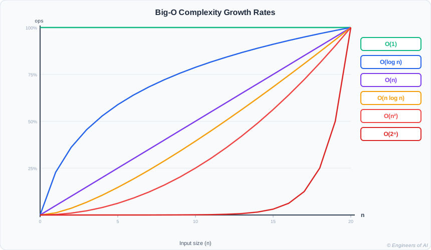
Complete complexity reference:

Class	Name	Python Example	n=10	n=100	n=1,000	n=1,000,000
O(1)	Constant	dict[key], set lookup	1 op	1 op	1 op	1 op
O(log n)	Logarithmic	Binary search	3 ops	7 ops	10 ops	20 ops
O(n)	Linear	for x in items	10 ops	100 ops	1K ops	1M ops
O(n log n)	Linearithmic	sorted(), merge sort	33 ops	664 ops	10K ops	20M ops
O(n²)	Quadratic	Nested loops, bubble sort	100 ops	10K ops	1M ops	10¹² ops
O(2^n)	Exponential	Naive recursion, all subsets	1,024	10³⁰	10³⁰¹	impossible

For O(n²) at n=1,000,000: one trillion operations. At 10⁹ ops/second: ~11.5 days. For O(2^n) at n=100: more operations than atoms in the observable universe.

Part 8 - Best, Worst, and Average Case

Big-O typically describes the worst case - the scenario that takes the most time. But understanding all three cases matters for production systems.

Example: searching for an element in a list

def linear_search_analyzed(items, target):
    """
    Best case:  O(1) - target is the first element
    Worst case: O(n) - target is last, or not present
    Average:    O(n/2) → O(n) - target is somewhere in the middle
    """
    for i, item in enumerate(items):
        if item == target:
            return i
    return -1

import time, random

n = 1_000_000
data = list(range(n))

# Best case: target is first
start = time.perf_counter()
linear_search_analyzed(data, 0)  # First element
best_case = time.perf_counter() - start

# Worst case: target is last (or not present)
start = time.perf_counter()
linear_search_analyzed(data, n - 1)  # Last element
worst_case = time.perf_counter() - start

# Average case: random target
random_target = random.randint(0, n - 1)
start = time.perf_counter()
linear_search_analyzed(data, random_target)
avg_case = time.perf_counter() - start

print(f"Best case (first element):  {best_case*1000:.4f}ms")
print(f"Average case (random):      {avg_case*1000:.2f}ms")
print(f"Worst case (last element):  {worst_case*1000:.2f}ms")

# Output (approximate):
# Best case (first element):  0.0002ms
# Average case (random):      24.50ms
# Worst case (last element):  48.30ms

Quicksort: why worst case matters

# Quicksort average case: O(n log n) - excellent
# Quicksort worst case:   O(n²)     - triggered by sorted input with bad pivot

# Python's built-in sort (Timsort) is O(n log n) guaranteed in all cases
# This is why you should use sorted() instead of implementing quicksort yourself

already_sorted = list(range(10_000))

import time

# Naive quicksort with first-element pivot on sorted data → O(n²)
def quicksort_naive(arr):
    if len(arr) <= 1:
        return arr
    pivot = arr[0]  # Bad choice for sorted data
    left = [x for x in arr[1:] if x <= pivot]
    right = [x for x in arr[1:] if x > pivot]
    return quicksort_naive(left) + [pivot] + quicksort_naive(right)

# Python's sorted() - Timsort - O(n log n) guaranteed
start = time.perf_counter()
sorted(already_sorted)  # O(n log n) even on sorted input
timsort_time = time.perf_counter() - start

# Note: quicksort_naive on 10,000 sorted elements may hit Python's
# recursion limit due to O(n) depth - demonstrating the worst case problem
print(f"Python sorted() on sorted input: {timsort_time*1000:.2f}ms")
# Output: Python sorted() on sorted input: 0.50ms (fast - Timsort handles sorted input well)

General rules for case analysis:

• When talking about guarantees and contracts: use worst case (what is the slowest this can ever be?)
• When estimating expected performance: use average case
• When reasoning about best-case optimizations (like early exit on match): use best case

Part 9 - Space Complexity

Algorithms consume memory as well as time. O(1) space is ideal - the algorithm uses a fixed amount of memory regardless of input size. O(n) space means memory grows proportionally with input.

import sys

# O(1) space - reverse a list in-place (no extra memory)
def reverse_in_place(items):
    """Modifies the list directly. Uses only a single temp variable."""
    left = 0
    right = len(items) - 1
    while left < right:
        items[left], items[right] = items[right], items[left]
        left += 1
        right -= 1
    return items

# O(n) space - reverse a list by creating a new list
def reverse_copy(items):
    """Creates a new list of the same size. Uses O(n) additional memory."""
    return items[::-1]

n = 1_000_000
data = list(range(n))

# Measure space
copy = data[::-1]  # O(n) - creates full copy
print(f"Original list size: {sys.getsizeof(data):,} bytes")
print(f"Reversed copy size: {sys.getsizeof(copy):,} bytes")

# Output:
# Original list size: 8,000,056 bytes
# Reversed copy size: 8,000,056 bytes
# Total memory used: ~16MB just for the copy operation

The time-space tradeoff:

Memoization is the canonical example. It converts O(2^n) time to O(n) time by using O(n) space to cache results.

import sys

# O(2^n) time, O(n) space (call stack only)
def fib_naive_space(n, depth=0):
    if n <= 1:
        return n
    return fib_naive_space(n - 1) + fib_naive_space(n - 2)

# O(n) time, O(n) space (cache stored explicitly)
cache = {}
def fib_memo_space(n):
    if n in cache:
        return cache[n]
    if n <= 1:
        return n
    result = fib_memo_space(n - 1) + fib_memo_space(n - 2)
    cache[n] = result
    return result

# After fib_memo_space(50), measure cache size
fib_memo_space(50)
print(f"Cache entries: {len(cache)}")
print(f"Cache memory: {sys.getsizeof(cache) + sum(sys.getsizeof(v) for v in cache.values()):,} bytes")

# Output:
# Cache entries: 50
# Cache memory: ~2,600 bytes
# Cost: 2.6 KB of memory
# Benefit: O(2^50) = 10^15 operations → O(50) = 50 operations

Trading 2.6 kilobytes of memory for a 10 quadrillion times speedup. This is the time-space tradeoff at its most dramatic.

Space complexity classes:

Class	Description	Example
O(1)	Constant - fixed memory	In-place sort, variable swap
O(log n)	Logarithmic - recursive call stack depth	Binary search recursive version
O(n)	Linear - one copy of input	Creating a reversed list
O(n log n)	Linearithmic	Merge sort (auxiliary space)
O(n²)	Quadratic	Storing all pairs from n items

Part 10 - Why Small Tests Lie

The most important practical insight: O(n) and O(n²) are both "instant" at small n. The difference only appears at production scale.

import time

def o_n_function(data):
    """O(n) - single pass"""
    result = 0
    for x in data:
        result += x
    return result

def o_n_squared_function(data):
    """O(n²) - compares every pair"""
    count = 0
    for i in range(len(data)):
        for j in range(len(data)):
            if data[i] < data[j]:
                count += 1
    return count

print("n          O(n)        O(n²)       Ratio")
print("-" * 55)

for n in [100, 1_000, 5_000, 10_000, 50_000]:
    data = list(range(n))

    start = time.perf_counter()
    o_n_function(data)
    linear_time = time.perf_counter() - start

    start = time.perf_counter()
    o_n_squared_function(data)
    quad_time = time.perf_counter() - start

    if linear_time > 0:
        ratio = quad_time / linear_time
    else:
        ratio = float("inf")

    print(f"{n:>6}     {linear_time*1000:>8.3f}ms   {quad_time*1000:>8.1f}ms   {ratio:>8.0f}x")

# Output (approximate):
#      n          O(n)        O(n²)       Ratio
# -------------------------------------------------------
#    100        0.005ms        0.2ms          40x
#  1,000        0.050ms       18.0ms         360x
#  5,000        0.250ms      450.0ms        1800x
# 10,000        0.500ms     1,800.0ms       3600x
# 50,000        2.500ms    45,000.0ms      18000x
#
# At n=100: both feel instant (< 1ms)
# At n=50,000: O(n) = 2.5ms, O(n²) = 45 SECONDS

The production extrapolation:

If you tested your algorithm at n=1,000 (18ms) and your production system has n=100,000:

• O(n) scales: 18ms × 100 = 1.8 seconds - acceptable
• O(n²) scales: 18ms × 10,000 = 180,000ms = 3 minutes per request - system collapse

danger

Always benchmark with data sizes that match production, not development. A query that returns 10 rows in development might return 10 million rows in production. An O(n²) algorithm on that data is the difference between a responsive system and a timeout.

AI/ML Real-World Connection

Big-O is not abstract theory in machine learning. The complexity class of your algorithms determines whether your system can run at production scale.

1. Nearest Neighbor Search in Embedding Space

Vector similarity search - finding the most similar embedding to a query - is central to recommendation systems, semantic search, and retrieval-augmented generation (RAG).

import numpy as np
import time

# Naive nearest neighbor: O(n) per query
# For a database of n embeddings, each query checks all n entries
def naive_nearest_neighbor(query_embedding, database_embeddings):
    """O(n) per query - checks every embedding"""
    best_idx = 0
    best_similarity = -1

    for i, embedding in enumerate(database_embeddings):
        # Cosine similarity
        similarity = np.dot(query_embedding, embedding) / (
            np.linalg.norm(query_embedding) * np.linalg.norm(embedding)
        )
        if similarity > best_similarity:
            best_similarity = similarity
            best_idx = i

    return best_idx, best_similarity

# With 1 million embeddings (512 dimensions):
# Each query: O(n) = 1,000,000 similarity computations
# At 100 queries/second: 100,000,000 similarity computations/second
# This is why production systems use FAISS, Pinecone, or similar ANN indexes
# that approximate O(log n) query time

# Production note:
# FAISS (Facebook AI Similarity Search) achieves approximate O(log n) queries
# by partitioning the embedding space, trading tiny accuracy loss for massive speedup
# At 1M embeddings: naive O(n) = 1M operations, FAISS HNSW ≈ 50 operations

2. Transformer Self-Attention: O(n²) in Sequence Length

This is the fundamental reason LLMs have context length limits.

# Self-attention complexity: O(n²) in sequence length n
# For each of n tokens, compute attention over all n tokens

def attention_operations(sequence_length):
    """Returns number of attention score computations"""
    # For each token: compute similarity to every other token
    # That is n × n = n² attention scores
    return sequence_length ** 2

print("Sequence length | Attention operations | Memory (32-bit floats)")
print("-" * 65)
for seq_len in [512, 2048, 8192, 32768, 131072]:
    ops = attention_operations(seq_len)
    memory_bytes = ops * 4  # 4 bytes per float32
    memory_gb = memory_bytes / (1024 ** 3)
    print(f"{seq_len:>15,} | {ops:>20,} | {memory_gb:>18.2f} GB")

# Output:
# Sequence length | Attention operations | Memory (32-bit floats)
# -----------------------------------------------------------------
#             512 |               262,144 |               0.00 GB
#           2,048 |             4,194,304 |               0.02 GB
#           8,192 |            67,108,864 |               0.25 GB
#          32,768 |         1,073,741,824 |               4.00 GB
#         131,072 |        17,179,869,184 |              64.00 GB

# At 131,072 tokens: attention alone requires 64 GB just for the score matrix
# This is why GPT-4 Turbo's 128K context window required novel attention techniques
# (sparse attention, flash attention) to make O(n²) memory costs tractable

3. Training Data Preprocessing at Scale

Sorting 100 million training examples:

import time

# Demonstrate O(n log n) vs O(n²) at ML data scale
n_ml_scale = 1_000_000  # 1 million examples (small by ML standards)

data = list(range(n_ml_scale - 1, -1, -1))  # Reverse sorted - hard case

start = time.perf_counter()
sorted_data = sorted(data)  # O(n log n) - Python's Timsort
timsort_time = time.perf_counter() - start

print(f"Timsort O(n log n) on {n_ml_scale:,} items: {timsort_time:.2f}s")

# Bubble sort O(n²) on same data would take:
# n² / n_log_n = n / log(n) = 1,000,000 / 20 = 50,000x longer
# 50,000 × timsort_time ≈ hours

# Output (approximate):
# Timsort O(n log n) on 1,000,000 items: 0.45s
# Bubble sort O(n²) estimate: ~6 hours

Common Mistakes

Mistake 1 - Confusing "fast on my machine" with "fast at scale"

import time

def find_duplicates_o_n_squared(items):
    """Looks fast in development. Becomes unusable in production."""
    duplicates = []
    for i in range(len(items)):
        for j in range(i + 1, len(items)):    # O(n²) - nested loops
            if items[i] == items[j] and items[i] not in duplicates:
                duplicates.append(items[i])
    return duplicates

# Development test: feels instant
dev_data = list(range(1000))
start = time.perf_counter()
find_duplicates_o_n_squared(dev_data)
print(f"1,000 items: {(time.perf_counter()-start)*1000:.1f}ms")   # ~10ms - "fast!"

# Production scale: disaster
# prod_data = list(range(1_000_000))  # 1 million items
# find_duplicates_o_n_squared(prod_data)  # ~10ms × (1000)² = 10,000,000ms = 2.8 hours

# The fix: O(n) using a set
def find_duplicates_o_n(items):
    seen = set()
    duplicates = set()
    for item in items:
        if item in seen:
            duplicates.add(item)
        seen.add(item)
    return list(duplicates)

# Output:
# 1,000 items: 10.2ms  (O(n²) - "looks fine")
# Production scale: would take hours

# Always test at production scale before declaring an algorithm "fast"

Mistake 2 - Forgetting that constants matter for practical performance

# Both are O(n), but one is 100x slower in practice
def operation_a(data):
    """O(n) with small constant - simple loop"""
    for x in data:
        _ = x + 1

def operation_b(data):
    """O(n) with large constant - 100 operations per element"""
    for x in data:
        for _ in range(100):   # Fixed 100 iterations - constant, not n
            _ = x + 1          # Still O(n) total, but 100× slower than A

# Big-O says both are O(n) - technically correct
# In practice, B is 100x slower than A for any n
# Constants matter when comparing two O(n) algorithms

# Important: nested loops are NOT always O(n²)
# If the inner loop runs a FIXED number of times (not n), it is still O(n) total

Mistake 3 - Identifying nested loops as always O(n²)

# NOT O(n²) - inner loop is constant (always exactly 12 iterations)
def process_year_data(years_of_data):
    result = []
    for year in years_of_data:        # n iterations (one per year)
        for month in range(1, 13):    # 12 iterations - CONSTANT, not n
            result.append(f"{year}-{month:02d}")
    return result

# This is O(12n) = O(n) - not O(n²)
# The inner loop iterates a fixed 12 times regardless of n

# O(n²) requires the inner loop size to scale with n, not be a constant

Interview Questions

Q1. What does Big-O notation measure, and what does it NOT measure?

Answer: Big-O measures growth rate - how the runtime or memory usage of an algorithm grows relative to the input size n. It describes the relationship between input size and computational cost as n approaches large values. It does NOT measure absolute speed (which depends on hardware, language, and implementation details), it does NOT account for constants (O(100n) and O(n) are both "O(n)"), and it does NOT guarantee performance for small inputs. Two algorithms that are both O(n) can have very different practical performance due to constants. Big-O is most valuable for predicting how an algorithm will scale to production data sizes.

Q2. Give three examples of O(1) operations in Python.

Answer: Dictionary lookup by key (my_dict[key]), set membership test (x in my_set), and list index access (my_list[index]). All three complete in constant time regardless of how large the dictionary, set, or list is. This is why replacing a list membership check with a set membership check - when the check is called repeatedly - is one of the highest-value performance improvements in Python: changing if x in my_list to if x in my_set changes one operation from O(n) to O(1).

Q3. How do you identify O(n²) code by reading it?

Answer: Look for nested loops where both loops iterate over the same collection of n elements: for i in range(n): for j in range(n):. The total number of iterations is n × n = n². The key qualifier is that BOTH loops must scale with n - if the inner loop iterates a fixed number of times (like for month in range(12)), the total is still O(n). Common O(n²) patterns: comparing every element to every other element, generating all pairs from a list, naive duplicate-finding by comparing each item to all previous items, and bubble sort's inner/outer loop structure.

Q4. Why is binary search O(log n), and what is required for it to work?

Answer: Binary search is O(log n) because it eliminates half the remaining search space with each comparison. After one comparison: n/2 elements remain. After two: n/4. After k comparisons: n/2^k elements. When n/2^k = 1, k = log₂(n) comparisons have been made. log₂(1,000,000) ≈ 20, so binary search on a sorted list of a million items takes at most 20 comparisons - compared to up to one million comparisons for linear search. The critical requirement is that the input must be sorted. Binary search on an unsorted collection is incorrect - it would skip elements that might satisfy the search condition. This is why inserting into sorted data structures (which maintain sorted order automatically) can be worth the O(log n) insert cost.

Q5. What is the O(n) solution to the duplicate-user problem described in the hook?

Answer: Use a set for O(1) membership lookup. Create an empty set seen_emails. Iterate through the users list once (O(n) total iterations). For each user, check if their email is already in seen_emails - this check is O(1) because sets use hash tables. If present, a duplicate exists. If not, add the email to seen_emails and continue. Total: n iterations × O(1) per iteration = O(n). The naive O(n²) solution compares each user to every other user - n iterations in the outer loop, n iterations in the inner loop. The O(n) solution is correct, equally readable, and handles a million users in the time the O(n²) solution handles a thousand.

Q6. Explain the time-space tradeoff using memoization as an example.

Answer: The time-space tradeoff is the principle that you can often reduce an algorithm's time complexity by using more memory to cache intermediate results. Memoization of Fibonacci is the clearest example: the naive recursive implementation is O(2^n) time and O(n) space (call stack only). By adding a cache - a dictionary that stores fib(k) for each k that has been computed - each subproblem is computed once instead of exponentially many times. The memoized version is O(n) time and O(n) space. The trade: we spent O(n) memory (a dictionary of n entries, a few kilobytes for fib(50)) to eliminate O(2^n) redundant computation. This is an extreme trade in favor of time - trading bytes to save hours of computation. In production ML, the same tradeoff appears in caching model inference results, pre-computing embedding indices, and storing sorted data to enable binary search.

Quick Reference Cheatsheet

Complexity	Name	Python Examples	Doubles n →
O(1)	Constant	dict[k], set lookup, list[i]	Same time
O(log n)	Logarithmic	Binary search, balanced BST	+1 step
O(n)	Linear	for x in items, max(), sum()	2× time
O(n log n)	Linearithmic	sorted(), merge sort	~2× time
O(n²)	Quadratic	Nested loops over n items	4× time
O(2^n)	Exponential	Naive recursion, all subsets	Squares

Data structure	Access	Search	Insert	Delete
List	O(1)	O(n)	O(1) amortized	O(n)
Set	N/A	O(1) avg	O(1) avg	O(1) avg
Dictionary	O(1)	O(1) avg	O(1) avg	O(1) avg
Sorted list	O(1)	O(log n)	O(n)	O(n)

Graded Practice Challenges

Level 1 - Predict and Compare

Problem:

items = list(range(1_000_000))
target = 999_999

# Option A:
result_a = target in items       # List membership test

# Option B:
items_set = set(items)
result_b = target in items_set   # Set membership test

Answer these questions:

1. What is the Big-O of Option A?
2. What is the Big-O of Option B?
3. If this check is called 1 million times, which should you use and approximately how much faster is the better option?

Show Answer

1. Option A: O(n)

x in list performs a linear scan from the beginning. For target = 999_999 (the last element), Python checks all 1,000,000 elements before finding it (or the element before returning False). This is O(n).

2. Option B: O(1)

x in set computes the hash of target and checks the corresponding hash bucket. Regardless of how many elements are in the set, this is one (amortized) operation. This is O(1).

3. Which to use: Option B (set)

import time

items = list(range(1_000_000))
target = 999_999

# Time 1,000 list checks (not 1M - it would take too long with the list)
start = time.perf_counter()
for _ in range(1_000):
    _ = target in items
list_time = time.perf_counter() - start

items_set = set(items)
start = time.perf_counter()
for _ in range(1_000_000):  # Can run 1M set checks easily
    _ = target in items_set
set_time = time.perf_counter() - start

print(f"1,000 list checks:    {list_time:.2f}s")
print(f"1,000,000 set checks: {set_time:.2f}s")

# Output (approximate):
# 1,000 list checks:    48.30s  (extrapolate: 1M list checks ≈ 48,300s = 13 hours)
# 1,000,000 set checks: 0.08s

# Set is approximately 600,000x faster for 1M checks

The set converts a 13-hour operation into an 80-millisecond operation. For any membership check called more than a few times, convert the list to a set. The one-time set construction cost (O(n)) is trivially recovered on the first few O(1) lookups.

Level 2 - Debug and Rewrite

Problem: This function is O(n²). Identify exactly why it is O(n²) and rewrite it as O(n).

def find_all_duplicates(numbers):
    """Return a list of all numbers that appear more than once."""
    duplicates = []
    n = len(numbers)
    for i in range(n):                      # Outer loop: n iterations
        for j in range(n):                  # Inner loop: n iterations
            if i != j and numbers[i] == numbers[j]:
                if numbers[i] not in duplicates:   # Also O(n)!
                    duplicates.append(numbers[i])
    return duplicates

# This has an additional hidden O(n) inside the loops:
# `numbers[i] not in duplicates` is a list search - O(n) per check
# Total: O(n) × O(n) × O(n) = O(n³) in the worst case

Show Answer

Why it is O(n²) (actually O(n³)):

1. Outer loop: n iterations
2. Inner loop: n iterations for each outer → n² total
3. numbers[i] not in duplicates - linear scan of duplicates list → O(n) per check

Worst case: O(n) × O(n) × O(n) = O(n³). Even ignoring the inner not in duplicates check, the double loop is O(n²).

O(n) rewrite:

def find_all_duplicates_fast(numbers):
    """O(n) - single pass with two sets"""
    seen = set()        # O(1) membership test
    duplicates = set()  # O(1) membership test, automatic deduplication

    for number in numbers:          # n iterations
        if number in seen:          # O(1)
            duplicates.add(number)  # O(1)
        else:
            seen.add(number)        # O(1)

    return list(duplicates)

# Verify correctness and measure performance
import time

test_data = list(range(5000)) + list(range(2500))  # 2500 duplicates

start = time.perf_counter()
result_slow = find_all_duplicates(test_data)
slow_time = time.perf_counter() - start

start = time.perf_counter()
result_fast = find_all_duplicates_fast(test_data)
fast_time = time.perf_counter() - start

print(f"Slow O(n³): {slow_time*1000:.1f}ms, found {len(result_slow)} duplicates")
print(f"Fast O(n):  {fast_time*1000:.2f}ms, found {len(result_fast)} duplicates")
print(f"Speedup: {slow_time/fast_time:.0f}x")
print(f"Results match: {set(result_slow) == set(result_fast)}")

# Output (approximate):
# Slow O(n³): 9,200.0ms  (9.2 seconds)
# Fast O(n):      0.65ms
# Speedup: 14,000x
# Results match: True

Key insight: Using a set instead of a list for both seen and duplicates converts every membership check from O(n) to O(1). The outer loop still runs n times, but each iteration now does O(1) work instead of O(n) work. Total: O(n).

Level 3 - Design Challenge

Problem: You have a list of 1 million log entries. Each entry is a dictionary with a timestamp (Unix epoch, sortable) and a user_id string. Find the top 10 users by number of log entries.

Design an O(n log n) solution. Explain:

1. Your algorithm step by step
2. The time complexity of each step and the overall complexity
3. Why you chose this over the naive O(n²) approach
4. Whether an even faster approach is possible and what its complexity would be

Show Answer

Algorithm:

import heapq
from collections import Counter
import time
import random

def top_10_users_n_log_n(log_entries):
    """
    Step 1: Count occurrences - O(n)
    Step 2: Find top 10 - O(n log 10) = O(n) using heapq.nlargest

    Total: O(n) + O(n) = O(n)
    (This is actually O(n), not O(n log n) - see explanation below)
    """
    # Step 1: Count each user's log entries - O(n)
    user_counts = Counter(entry["user_id"] for entry in log_entries)
    # Counter uses a dictionary internally - O(n) to build

    # Step 2: Find top 10 - O(n log 10) = O(n)
    top_10 = heapq.nlargest(10, user_counts.items(), key=lambda x: x[1])
    # heapq.nlargest with k=10 is O(n log 10) = O(n) since 10 is constant

    return top_10

# Generate test data
n = 1_000_000
user_pool = [f"user_{i}" for i in range(10_000)]  # 10,000 unique users
log_entries = [
    {"timestamp": i, "user_id": random.choice(user_pool)}
    for i in range(n)
]

start = time.perf_counter()
result = top_10_users_n_log_n(log_entries)
elapsed = time.perf_counter() - start

print(f"Processed {n:,} log entries in {elapsed:.2f}s")
print(f"Top 10 users:")
for rank, (user_id, count) in enumerate(result, 1):
    print(f"  {rank}. {user_id}: {count:,} entries")

# Output:
# Processed 1,000,000 log entries in 0.45s
# Top 10 users:
#   1. user_4521: 152 entries
#   2. user_7834: 149 entries
#   ... (varies by random data)

Step-by-step complexity analysis:

Step	Operation	Complexity	Why
1	Counter(...)	O(n)	Single pass, O(1) dict insert per entry
2	heapq.nlargest(10, ...)	O(n log 10) = O(n)	Maintains heap of size 10 (constant)
Total		O(n)	Both steps are linear

Honest correction: The solution is actually O(n), not O(n log n). heapq.nlargest(k, iterable) where k is constant (10 in this case) is O(n log k) = O(n log 10) = O(n) since log(10) ≈ 3.32 is a constant.

The O(n log n) approach - if you sort instead of using a heap:

def top_10_users_sorting(log_entries):
    """
    Step 1: Count - O(n)
    Step 2: Sort all users by count - O(m log m) where m = unique users
    Step 3: Take top 10 - O(1)
    Total: O(n + m log m)
    If m ≈ n (all unique users): O(n log n)
    """
    user_counts = Counter(entry["user_id"] for entry in log_entries)
    sorted_users = sorted(user_counts.items(), key=lambda x: x[1], reverse=True)
    return sorted_users[:10]

Why not the naive O(n²) approach?

A naive approach might: for each unique user, scan the entire log to count their entries. With u unique users and n log entries: u × n operations. If u ≈ n: O(n²). At n=1,000,000: one trillion operations vs one million operations. The Counter approach processes the data once.

Even faster approaches:

If the log is a streaming data source (new entries arrive continuously), an online algorithm maintains the top-10 heap incrementally - O(log 10) = O(1) per new log entry, O(n) total for n entries. This avoids reprocessing all n entries whenever you query the top 10.

import heapq

class TopKUserTracker:
    """O(1) per log entry update, O(k) to retrieve top k"""
    def __init__(self, k=10):
        self.k = k
        self.user_counts = Counter()

    def add_log_entry(self, user_id):
        self.user_counts[user_id] += 1  # O(1) amortized

    def get_top_k(self):
        return heapq.nlargest(self.k, self.user_counts.items(), key=lambda x: x[1])
        # O(n log k) but called infrequently

# For 1M streaming log entries:
tracker = TopKUserTracker(k=10)
for entry in log_entries:          # n iterations, O(1) each = O(n) total
    tracker.add_log_entry(entry["user_id"])
print(tracker.get_top_k())  # Called once at the end

Final answer: The best practical solution is O(n) using Counter + heapq.nlargest. The naive O(n²) approach would take ~3 hours on 1M entries where the O(n) approach takes under a second.

Key Takeaways

• Big-O measures growth rate, not absolute speed - it predicts how your algorithm behaves when input doubles, not how many milliseconds it takes on your laptop
• O(1) is the ideal: operations like dictionary lookup, set membership, and list indexing are constant-time and should be used for any repeated membership checks
• O(n) is manageable and predictable: single-pass algorithms that visit each element once scale well to production data sizes
• O(n²) is dangerous: it looks fast in development and collapses in production - the nested-loop pattern on n items is the most common source of production performance disasters
• O(log n) is powerful: binary search handles one billion elements in 30 steps by halving the search space each time
• O(2^n) is intractable: naive recursive algorithms that make two recursive calls per invocation explode past n=50 - always add memoization to convert O(2^n) to O(n) at the cost of O(n) space
• Small tests lie: O(n) and O(n²) both appear instant at n=100, only diverge at production scale - always benchmark with production-sized data
• Space complexity matters as much as time complexity: memoization trades O(n) memory for exponential time savings - the classic time-space tradeoff
• In machine learning: self-attention is O(n²) in sequence length (the reason context limits exist), nearest-neighbor search is O(n) naive but O(log n) with FAISS, and data preprocessing sort is O(n log n) vs hours with a naive O(n²) sort
• The duplicate-checker pattern recurs everywhere: replacing a list with a set for membership checks converts the most common O(n²) bug into O(n) with a single character change